Graphics of the Multiple Comparisons with agricolae

Felipe de Mendiburu¹, Muhammad Yaseen²

2020-05-02

1. Professor of the Academic Department of Statistics and Informatics of the Faculty of Economics and Planning.National University Agraria La Molina-PERU.

2. Department of Mathematics and Statistics, University of Agriculture Faisalabad, Pakistan.

Graphics of the multiple comparison

The results of a comparison can be graphically seen with the functions bar.group, bar.err and diffograph.

bar.group

A function to plot horizontal or vertical bar, where the letters of groups of treatments is expressed. The function applies to all functions comparison treatments. Each object must use the group object previously generated by comparative function in indicating that group = TRUE.

Example

# model <-aov (yield ~ fertilizer, data = field) 
# out <-LSD.test (model, "fertilizer", group = TRUE) 
# bar.group (out$group)
str(bar.group)

function (x, horiz = FALSE, ...)  

The Median test with option group=TRUE (default) is used in the exercise.

bar.err

A function to plot horizontal or vertical bar, where the variation of the error is expressed in every treatments. The function applies to all functions comparison treatments. Each object must use the means object previously generated by the comparison function, see Figure @ref(fig:f4)

# model <-aov (yield ~ fertilizer, data = field) 
# out <-LSD.test (model, "fertilizer", group = TRUE) 
# bar.err(out$means)
str(bar.err)

function (x, variation = c("SE", "SD", "range", "IQR"), horiz = FALSE, 
    bar = TRUE, ...)  

variation

SE: Standard error

SD: standard deviation

range: max-min

oldpar<-par(mfrow=c(2,2),mar=c(3,3,2,1),cex=0.7)
c1<-colors()[480]; c2=colors()[65]
data(sweetpotato)
model<-aov(yield~virus, data=sweetpotato)
outHSD<- HSD.test(model, "virus",console=TRUE)

Study: model ~ "virus"

HSD Test for yield 

Mean Square Error:  22.48917 

virus,  means

      yield      std r  Min  Max
cc 24.40000 3.609709 3 21.7 28.5
fc 12.86667 2.159475 3 10.6 14.9
ff 36.33333 7.333030 3 28.0 41.8
oo 36.90000 4.300000 3 32.1 40.4

Alpha: 0.05 ; DF Error: 8 
Critical Value of Studentized Range: 4.52881 

Minimun Significant Difference: 12.39967 

Treatments with the same letter are not significantly different.

      yield groups
oo 36.90000      a
ff 36.33333     ab
cc 24.40000     bc
fc 12.86667      c

bar.err(outHSD$means, variation="range",ylim=c(0,50),col=c1,las=1)
bar.err(outHSD$means, variation="IQR",horiz=TRUE, xlim=c(0,50),col=c2,las=1)
plot(outHSD, variation="range",las=1)

Warning in plot.group(outHSD, variation = "range", las = 1): NAs introduced by
coercion

plot(outHSD, horiz=TRUE, variation="SD",las=1)

Warning in plot.group(outHSD, horiz = TRUE, variation = "SD", las = 1): NAs
introduced by coercion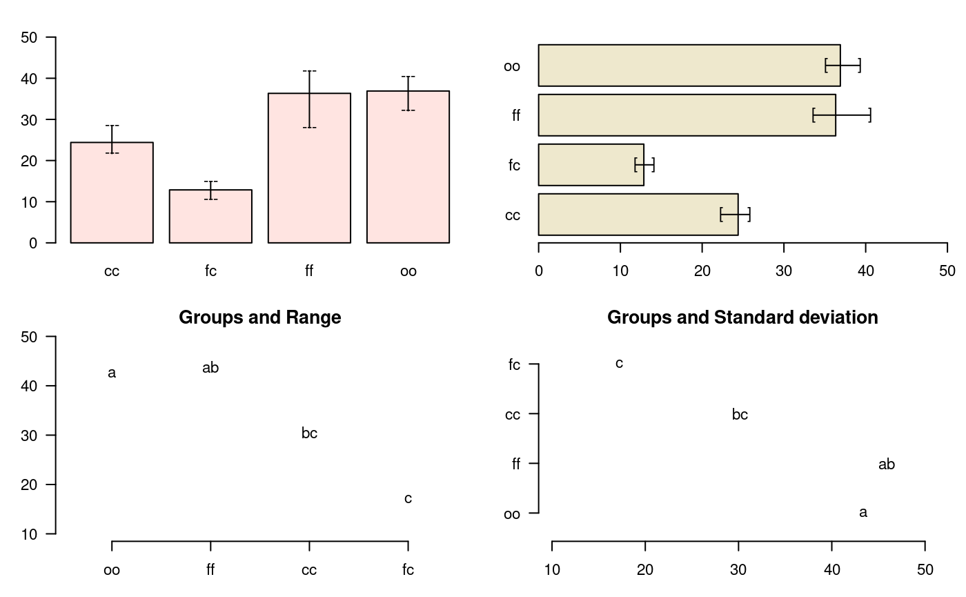

Comparison between treatments

par(oldpar)

oldpar<-par(mfrow=c(2,2),cex=0.7,mar=c(3.5,1.5,3,1))
C1<-bar.err(modelPBIB$means[1:7, ], ylim=c(0,9), col=0, main="C1",
variation="range",border=3,las=2)
C2<-bar.err(modelPBIB$means[8:15,], ylim=c(0,9), col=0, main="C2",
variation="range", border =4,las=2)
# Others graphic
C3<-bar.err(modelPBIB$means[16:22,], ylim=c(0,9), col=0, main="C3",
variation="range",border =2,las=2)
C4<-bar.err(modelPBIB$means[23:30,], ylim=c(0,9), col=0, main="C4",
variation="range", border =6,las=2)
# Lattice graphics
par(oldpar)
oldpar<-par(mar=c(2.5,2.5,1,0),cex=0.6)
bar.group(modelLattice$group,ylim=c(0,55),density=10,las=1)
par(oldpar)

plot.group

It plot groups and variation of the treatments to compare. It uses the objects generated by a procedure of comparison like LSD (Fisher), duncan, Tukey (HSD), Student Newman Keul (SNK), Scheffe, Waller-Duncan, Ryan, Einot and Gabriel and Welsch (REGW), Kruskal Wallis, Friedman, Median, Waerden and other tests like Durbin, DAU, BIB, PBIB. The variation types are range (maximun and minimun), IQR (interquartile range), SD (standard deviation) and SE (standard error), see Figure @ref(fig:f13).

The function: plot.group() and their arguments are x (output of test), variation = c("range", "IQR", "SE", "SD"), horiz (TRUE or FALSE), xlim, ylim and main are optional plot() parameters and others plot parameters.

# model : yield ~ virus
# Important group=TRUE
oldpar<-par(mfrow=c(1,2),mar=c(3,3,1,1),cex=0.8)
x<-duncan.test(model, "virus", group=TRUE)
plot(x,las=1)

Warning in plot.group(x, las = 1): NAs introduced by coercion

plot(x,variation="IQR",horiz=TRUE,las=1)

Warning in plot.group(x, variation = "IQR", horiz = TRUE, las = 1): NAs
introduced by coercion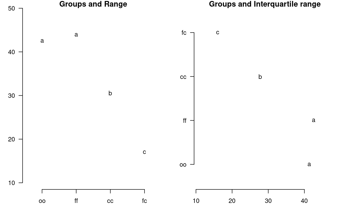

Grouping of treatments and its variation, Duncan method

par(oldpar)

diffograph

It plots bars of the averages of treatments to compare. It uses the objects generated by a procedure of comparison like LSD (Fisher), duncan, Tukey (HSD), Student Newman Keul (SNK), Scheffe, Ryan, Einot and Gabriel and Welsch (REGW), Kruskal Wallis, Friedman and Waerden (Hsu, 1996) see Figure @ref(fig:f5).

# function (x, main = NULL, color1 = "red", color2 = "blue", 
#    color3 = "black", cex.axis = 0.8, las = 1, pch = 20, 
#    bty = "l", cex = 0.8, lwd = 1, xlab = "", ylab = "", 
#   ...)
# model : yield ~ virus
# Important group=FALSE
x<-HSD.test(model, "virus", group=FALSE)
diffograph(x,cex.axis=0.9,xlab="Yield",ylab="Yield",cex=0.9)

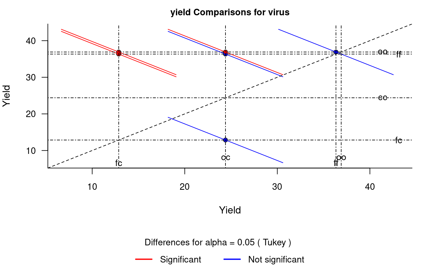
Mean-Mean scatter plot representation of the Tukey method

References

Hsu, J. C. (1996). Multiple Comparisons: Theory and Methods. Chapman; Hall/CRC.