Stability Analysis with agricolae
Felipe de Mendiburu1, Muhammad Yaseen2
2020-05-02
Source:vignettes/StabilityAnalysis.Rmd
StabilityAnalysis.Rmd
- Professor of the Academic Department of Statistics and Informatics of the Faculty of Economics and Planning.National University Agraria La Molina-PERU.
- Department of Mathematics and Statistics, University of Agriculture Faisalabad, Pakistan.
Stability Analysis
In agricolae there are two methods for the study of stability and the AMMI model. These are: a parametric model for a simultaneous selection in yield and stability “SHUKLA’S STABILITY VARIANCE AND KANG’S”, (Kang, 1993) and a non-parametric method of Haynes, based on the data range.
Parametric Stability
Use the parametric model, function stability.par.
Prepare a data table where the rows and the columns are the genotypes and the environments, respectively. The data should correspond to yield averages or to another measured variable. Determine the variance of the common error for all the environments and the number of repetitions that was evaluated for every genotype. If the repetitions are different, find a harmonious average that will represent the set. Finally, assign a name to each row that will represent the genotype (Kang, 1993). We will consider five environments in the following example:
options(digit=2)
f <- system.file("external/dataStb.csv", package="agricolae")
dataStb<-read.csv(f)
stability.par(dataStb, rep=4, MSerror=1.8, alpha=0.1, main="Genotype",console=TRUE)
 INTERACTIVE PROGRAM FOR CALCULATING SHUKLA'S STABILITY VARIANCE AND KANG'S
                        YIELD - STABILITY (YSi) STATISTICS
 Genotype
 Environmental index  - covariate

 Analysis of Variance

               Df    Sum Sq  Mean Sq F value Pr(>F)
Total         203 2964.1716
Genotypes      16  186.9082  11.6818    4.17 <0.001
Environments   11 2284.0116 207.6374  115.35 <0.001
Interaction   176  493.2518   2.8026    1.56 <0.001
Heterogeneity  16   44.8576   2.8036       1  0.459
Residual      160  448.3942   2.8025    1.56 <0.001
Pooled Error  576                1.8

 Genotype. Stability statistics

      Mean Sigma-square  . s-square  . Ecovalence
A 7.383333     2.474081 ns 2.449076 ns  25.826563
B 6.783333     1.600869 ns 1.434734 ns  17.351269
C 7.250000     0.567657 ns 0.633936 ns   7.323033
D 6.783333     2.611778 ns 2.134731 ns  27.163033
E 7.066667     1.862364 ns 2.047627 ns  19.889308
F 6.916667     3.575818  * 3.951442  *  36.519896
G 7.808333     3.580929  * 3.957319  *  36.569504
H 7.908333     2.723717 ns 2.118116 ns  28.249504
I 7.275000     4.248566 ** 3.936130  *  43.049504
J 7.083333     2.273838 ns 2.506382 ns  23.883033
K 6.433333     2.560384 ns 2.551518 ns  26.664210
L 6.891667     1.558061 ns 1.732557 ns  16.935779
M 6.791667     3.483879  * 3.275985 ns  35.627543
N 7.491667     5.164848 ** 4.875189 **  51.942837
O 7.658333     2.380202 ns 2.635025 ns  24.915386
P 6.425000     3.445414  * 3.713885  *  35.254210
Q 6.158333     3.531232  * 3.688232  *  36.087151


Signif. codes:  0 '**' 0.01 '*' 0.05 'ns' 1

Simultaneous selection for yield and stability  (++)

     Yield Rank Adj.rank Adjusted Stab.var Stab.rating YSi ...
A 7.383333   13        1       14 2.474081           0  14   +
B 6.783333    4       -1        3 1.600869           0   3
C 7.250000   11        1       12 0.567657           0  12   +
D 6.783333    4       -1        3 2.611778           0   3
E 7.066667    9        1       10 1.862364           0  10   +
F 6.916667    8       -1        7 3.575818          -4   3
G 7.808333   16        2       18 3.580929          -4  14   +
H 7.908333   17        2       19 2.723717           0  19   +
I 7.275000   12        1       13 4.248566          -8   5
J 7.083333   10        1       11 2.273838           0  11   +
K 6.433333    3       -2        1 2.560384           0   1
L 6.891667    7       -1        6 1.558061           0   6
M 6.791667    6       -1        5 3.483879          -4   1
N 7.491667   14        1       15 5.164848          -8   7   +
O 7.658333   15        2       17 2.380202           0  17   +
P 6.425000    2       -2        0 3.445414          -4  -4
Q 6.158333    1       -3       -2 3.531232          -4  -6

 Yield Mean: 7.065196
 YS    Mean: 6.823529
 LSD (0.05): 0.4511874
 - - - - - - - - - - -
 +   selected genotype
 ++  Reference: Kang, M. S. 1993. Simultaneous selection for yield
 and stability: Consequences for growers. Agron. J. 85:754-757.
For 17 genotypes, the identification is made by letters. An error variance of 2 and 4 repetitions is assumed.
Analysis
output <- stability.par(dataStb, rep=4, MSerror=2)
names(output)
[1] "analysis" "statistics" "stability" print(output$stability)
     Yield Rank Adj.rank Adjusted Stab.var Stab.rating YSi ...
A 7.383333   13        1       14 2.474081           0  14   +
B 6.783333    4       -1        3 1.600869           0   3
C 7.250000   11        1       12 0.567657           0  12   +
D 6.783333    4       -1        3 2.611778           0   3
E 7.066667    9        1       10 1.862364           0  10   +
F 6.916667    8       -1        7 3.575818          -2   5
G 7.808333   16        2       18 3.580929          -2  16   +
H 7.908333   17        2       19 2.723717           0  19   +
I 7.275000   12        1       13 4.248566          -4   9   +
J 7.083333   10        1       11 2.273838           0  11   +
K 6.433333    3       -2        1 2.560384           0   1
L 6.891667    7       -1        6 1.558061           0   6
M 6.791667    6       -1        5 3.483879          -2   3
N 7.491667   14        1       15 5.164848          -8   7
O 7.658333   15        2       17 2.380202           0  17   +
P 6.425000    2       -2        0 3.445414          -2  -2
Q 6.158333    1       -2       -1 3.531232          -2  -3
The selected genotypes are: A, C, E, G, H, I, J and O. These genotypes have a higher yield and a lower variation. to see output$analysis, the interaction is significant.
If for example there is an environmental index, it can be added as a covariate In the first five locations. For this case, the altitude of the localities is included.
data5<-dataStb[,1:5]
altitude<-c(1200, 1300, 800, 1600, 2400)
stability <- stability.par(data5,rep=4,MSerror=2, cova=TRUE, name.cov= "altitude",
file.cov=altitude)
Non-parametric Stability
For non-parametric stability, the function in agricolae is stability.nonpar(). The names of the genotypes should be included in the first column, and in the other columns, the response by environments (Haynes et al., 1998).
Analysis
data <- data.frame(name=row.names(dataStb), dataStb)
output<-stability.nonpar(data, "YIELD", ranking=TRUE)
names(output)
[1] "ranking" "statistics"output$statistics
      MEAN      es1 es2       vs1      vs2  chi.ind  chi.sum
1 7.065196 5.647059  24 0.7247475 46.72727 8.843605 27.58711
AMMI
The model AMMI uses the biplot constructed through the principal components generated by the interaction environment-genotype. If there is such interaction, the percentage of the two principal components would explain more than the 50% of the total variation; in such case, the biplot would be a good alternative to study the interaction environment-genotype (Crossa, 1990).
The data for AMMI should come from similar experiments conducted in different environments. Homogeneity of variance of the experimental error, produced in the different environments, is required. The analysis is done by combining the experiments.
The data can be organized in columns, thus: environment, genotype, repetition, and variable.
The data can also be the averages of the genotypes in each environment, but it is necessary to consider a harmonious average for the repetitions and a common variance of the error. The data should be organized in columns: environment, genotype, and variable.
When performing AMMI, this generates the Biplot, Triplot and Influence graphics, see Figure @ref(fig:f6).
For the application, we consider the data used in the example of parametric stability (study):
plot.AMMI structure, plot()
str(plot.AMMI)
[1] "ANOVA" "genXenv" "analysis" "means" "biplot" "PC" model$ANOVA
Analysis of Variance Table

Response: Y
           Df Sum Sq Mean Sq  F value    Pr(>F)
ENV         5 122284 24456.9 257.0382  9.08e-12 ***
REP(ENV)   12   1142    95.1   2.5694  0.002889 **
GEN        27  17533   649.4  17.5359 < 2.2e-16 ***
ENV:GEN   135  23762   176.0   4.7531 < 2.2e-16 ***
Residuals 324  11998    37.0
---
Signif. codes: 0 '***' 0.001 '**' 0.01 '*' 0.05 '.' 0.1 ' ' 1model$analysis
    percent  acum Df     Sum.Sq   Mean.Sq F.value   Pr.F
PC1    56.3  56.3 31 13368.5954 431.24501   11.65 0.0000
PC2    27.1  83.3 29  6427.5799 221.64069    5.99 0.0000
PC3     9.4  92.7 27  2241.9398  83.03481    2.24 0.0005
PC4     4.3  97.1 25  1027.5785  41.10314    1.11 0.3286
PC5     2.9 100.0 23   696.1012  30.26527    0.82 0.7059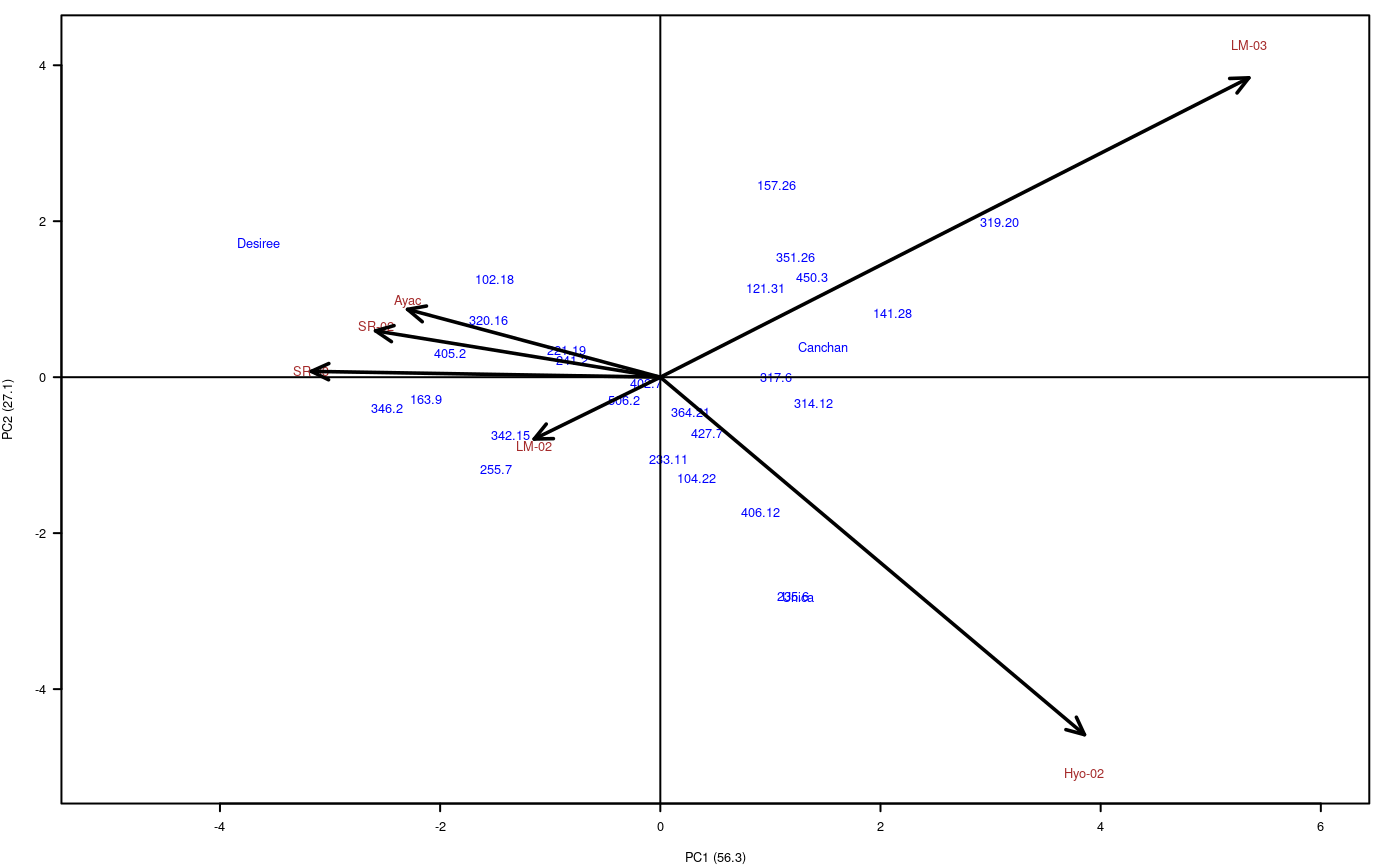
Biplot
par(oldpar)
In this case, the interaction is significant. The first two components explain 83.4 %; then the biplot can provide information about the interaction genotype-environment. With the triplot, 92.8% would be explained.
To triplot require klaR package. in R execute:
plot(model,type=2,las=1)
AMMI index and yield stability
Calculate AMMI stability value (ASV) and Yield stability index (YSI) (Purchase, 1997; N. et al., 2008).
data(plrv)
model<- with(plrv,AMMI(Locality, Genotype, Rep, Yield, console=FALSE))
index<-index.AMMI(model)
# Crops with improved stability according AMMI.
print(index[order(index[,3]),])
              ASV YSI rASV rYSI    means
402.7   0.2801470  20    1   19 27.47748
364.21  0.7236998  12    2   10 34.05974
506.2   0.7511331  14    3   11 33.26623
233.11  1.0582263  21    4   17 28.66655
427.7   1.1467970  12    5    7 36.19020
104.22  1.4627695  19    6   13 31.28887
241.2   1.6774241  29    7   22 26.34039
221.19  1.8014494  34    8   26 22.98480
317.6   2.1874274  18    9    9 35.32583
121.31  2.2937918  25   10   15 30.10174
406.12  2.5631734  23   11   12 32.68323
314.12  2.9170536  30   12   18 28.17335
342.15  2.9219360  37   13   24 26.01336
351.26  2.9786832  22   14    8 36.11581
Canchan 3.0975884  35   15   20 27.00126
450.3   3.1430174  22   16    6 36.19602
157.26  3.2923168  22   17    5 36.95181
320.16  3.3208950  39   18   21 26.34808
255.7   3.3289736  33   19   14 30.58975
102.18  3.3801820  43   20   23 26.31947
235.6   3.7647078  25   21    4 38.63477
Unica   3.8380782  24   22    2 39.10400
405.2   3.9832546  39   23   16 28.98663
163.9   4.4269636  51   24   27 21.41747
141.28  4.4672401  26   25    1 39.75624
346.2   5.1827747  51   26   25 23.84175
319.20  6.7164864  30   27    3 38.75767
Desiree 7.7833445 56 28 28 16.15569 ASV YSI rASV rYSI means
141.28 4.4672401 26 25 1 39.75624
Unica 3.8380782 24 22 2 39.10400
319.20 6.7164864 30 27 3 38.75767
235.6 3.7647078 25 21 4 38.63477
157.26 3.2923168 22 17 5 36.95181
450.3 3.1430174 22 16 6 36.19602
427.7 1.1467970 12 5 7 36.19020
351.26 2.9786832 22 14 8 36.11581
317.6 2.1874274 18 9 9 35.32583
364.21 0.7236998 12 2 10 34.05974
506.2 0.7511331 14 3 11 33.26623
406.12 2.5631734 23 11 12 32.68323
104.22 1.4627695 19 6 13 31.28887
255.7 3.3289736 33 19 14 30.58975
121.31 2.2937918 25 10 15 30.10174
405.2 3.9832546 39 23 16 28.98663
233.11 1.0582263 21 4 17 28.66655
314.12 2.9170536 30 12 18 28.17335
402.7 0.2801470 20 1 19 27.47748
Canchan 3.0975884 35 15 20 27.00126
320.16 3.3208950 39 18 21 26.34808
241.2 1.6774241 29 7 22 26.34039
102.18 3.3801820 43 20 23 26.31947
342.15 2.9219360 37 13 24 26.01336
346.2 5.1827747 51 26 25 23.84175
221.19 1.8014494 34 8 26 22.98480
163.9 4.4269636 51 24 27 21.41747
Desiree 7.7833445 56 28 28 16.15569References
Crossa, J. (1990). “Statistical Analyses of Multilocation Trials,” in Advances in agronomy (Elsevier), 55–85.
Haynes, K. G., Lambert, D. H., Christ, B. J., Weingartner, D. P., Douches, D. S., Backlund, J. E., et al. (1998). Phenotypic stability of resistance to late blight in potato clones evaluated at eight sites in the United Stated. 75, 211–217.
Kang, M. S. (1993). Phenotypic stability of resistance to late blight in potato clones evaluated at eight sites in the United Stated. Agronomy Journal 85, 754–757.
N., S., H.Sabaghpour, S., and Dehghani, H. (2008). The use of an AMMI model and its parameters to analyse yield stability in multienvironment trials. Journal of Agricultural Science 146, 571–581.
Purchase, J. L. (1997). Parametric analysis to describe genotype environment interaction and yield stability in winter wheat.