Example 5.2 from Experimental Design and Analysis for Tree Improvement
Source:R/Exam5.2.R
Exam5.2.RdExam5.2 presents the height of 37 seedlots from 6 sites.
References
E.R. Williams, C.E. Harwood and A.C. Matheson (2023). Experimental Design and Analysis for Tree Improvement. CSIRO Publishing (https://www.publish.csiro.au/book/3145/).
See also
Examples
library(car)
library(dae)
library(dplyr)
library(emmeans)
library(ggplot2)
library(lmerTest)
library(magrittr)
library(predictmeans)
library(supernova)
data(DataExam5.2)
fm5.7 <- lm(formula = Ht ~ Site*SeedLot, data = DataExam5.2)
# Pg. 77
anova(fm5.7)
#> Warning: ANOVA F-tests on an essentially perfect fit are unreliable
#> Analysis of Variance Table
#>
#> Response: Ht
#> Df Sum Sq Mean Sq F value Pr(>F)
#> Site 5 4157543 831509 NaN NaN
#> SeedLot 36 4425296 122925 NaN NaN
#> Site:SeedLot 150 1351054 9007 NaN NaN
#> Residuals 0 0 NaN
fm5.9 <- lm(formula = Ht ~ Site*SeedLot, data = DataExam5.2)
# Pg. 77
anova(fm5.9)
#> Warning: ANOVA F-tests on an essentially perfect fit are unreliable
#> Analysis of Variance Table
#>
#> Response: Ht
#> Df Sum Sq Mean Sq F value Pr(>F)
#> Site 5 4157543 831509 NaN NaN
#> SeedLot 36 4425296 122925 NaN NaN
#> Site:SeedLot 150 1351054 9007 NaN NaN
#> Residuals 0 0 NaN
ANOVAfm5.9 <- anova(fm5.9)
#> Warning: ANOVA F-tests on an essentially perfect fit are unreliable
ANOVAfm5.9[4, 1:3] <- c(384, 384*964, 964)
ANOVAfm5.9[3, 4] <- ANOVAfm5.9[3, 3]/ANOVAfm5.9[4, 3]
ANOVAfm5.9[3, 5] <- pf(
q = ANOVAfm5.9[3, 4]
, df1 = ANOVAfm5.9[3, 1]
, df2 = ANOVAfm5.9[4, 1]
, lower.tail = FALSE
)
# Pg. 77
ANOVAfm5.9
#> Analysis of Variance Table
#>
#> Response: Ht
#> Df Sum Sq Mean Sq F value Pr(>F)
#> Site 5 4157543 831509 NaN NaN
#> SeedLot 36 4425296 122925 NaN NaN
#> Site:SeedLot 150 1351054 9007 9.3434 < 2.2e-16 ***
#> Residuals 384 370176 964
#> ---
#> Signif. codes: 0 '***' 0.001 '**' 0.01 '*' 0.05 '.' 0.1 ' ' 1
Tab5.14 <-
DataExam5.2 %>%
summarise(Mean = mean(Ht, na.rm = TRUE), .by = SeedLot) %>%
left_join(
DataExam5.2 %>%
nest_by(SeedLot) %>%
mutate(fm2 = list(lm(Ht ~ SiteMean, data = data))) %>%
summarise(Slope = coef(fm2)[2])
, by = "SeedLot"
)
#> `summarise()` has grouped output by 'SeedLot'. You can override using the
#> `.groups` argument.
# Pg. 81
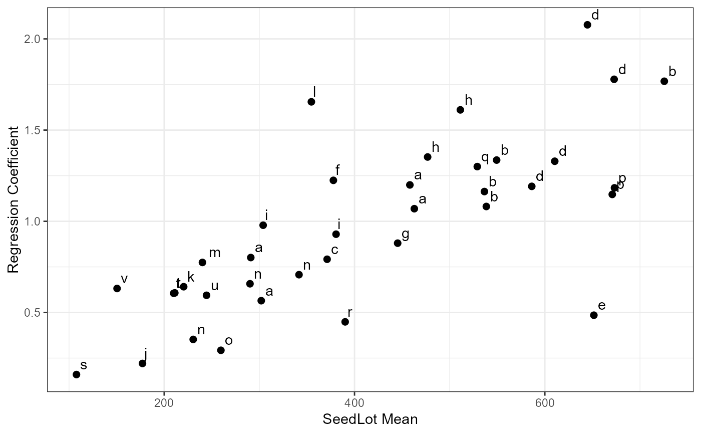
Tab5.14
#> # A tibble: 37 × 3
#> SeedLot Mean Slope
#> <fct> <dbl> <dbl>
#> 1 13877 291 0.801
#> 2 13866 302 0.565
#> 3 13689 463. 1.07
#> 4 13688 458. 1.20
#> 5 13861 538. 1.08
#> 6 13854 536. 1.16
#> 7 13686 726. 1.77
#> 8 13684 549. 1.34
#> 9 13864 371. 0.792
#> 10 13863 586. 1.19
#> # ℹ 27 more rows
DevSS2 <-
DataExam5.2 %>%
nest_by(SeedLot) %>%
mutate(fm2 = list(lm(Ht ~ SiteMean, data = data))) %>%
summarise(SSE = anova(fm2)[2, 2]) %>%
ungroup() %>%
summarise(Dev = sum(SSE)) %>%
as.numeric()
#> Warning: There were 2 warnings in `summarise()`.
#> The first warning was:
#> ℹ In argument: `SSE = anova(fm2)[2, 2]`.
#> ℹ In row 12.
#> Caused by warning in `anova.lm()`:
#> ! ANOVA F-tests on an essentially perfect fit are unreliable
#> ℹ Run `dplyr::last_dplyr_warnings()` to see the 1 remaining warning.
#> `summarise()` has grouped output by 'SeedLot'. You can override using the
#> `.groups` argument.
ANOVAfm5.9.1 <-
rbind(
ANOVAfm5.9[1:3, ]
, c(
ANOVAfm5.9[2, 1]
, ANOVAfm5.9[3, 2] - DevSS2
, (ANOVAfm5.9[3, 2] - DevSS2)/ANOVAfm5.9[2, 1]
, NA
, NA
)
, c(
ANOVAfm5.9[3, 1]-ANOVAfm5.9[2, 1]
, DevSS2
, DevSS2/(ANOVAfm5.9[3, 1]-ANOVAfm5.9[2, 1])
, DevSS2/(ANOVAfm5.9[3, 1]-ANOVAfm5.9[2, 1])/ANOVAfm5.9[4, 3]
, pf(
q = DevSS2/(ANOVAfm5.9[3, 1]-ANOVAfm5.9[2, 1])/ANOVAfm5.9[4, 3]
, df1 = ANOVAfm5.9[3, 1]-ANOVAfm5.9[2, 1]
, df2 = ANOVAfm5.9[4, 1]
, lower.tail = FALSE
)
)
, ANOVAfm5.9[4, ]
)
rownames(ANOVAfm5.9.1) <-
c("Site", "SeedLot", "Site:SeedLot", " regressions", " deviations", "Residuals")
# Pg. 82
ANOVAfm5.9.1
#> Analysis of Variance Table
#>
#> Response: Ht
#> Df Sum Sq Mean Sq F value Pr(>F)
#> Site 5 4157543 831509 NaN NaN
#> SeedLot 36 4425296 122925 NaN NaN
#> Site:SeedLot 150 1351054 9007 9.3434 < 2.2e-16 ***
#> regressions 36 703203 19533
#> deviations 114 647851 5683 5.8951 < 2.2e-16 ***
#> Residuals 384 370176 964
#> ---
#> Signif. codes: 0 '***' 0.001 '**' 0.01 '*' 0.05 '.' 0.1 ' ' 1
Code <- c("a","a","a","a","b","b","b","b","c","d","d","d","d","e","f","g",
"h","h","i","i","j","k","l","m","n","n","n","o","p","p","q","r",
"s","t","t","u","v")
Tab5.14$Code <- Code
ggplot(data = Tab5.14, mapping = aes(x = Mean, y = Slope))+
geom_point(size = 2) +
geom_text(aes(label = Code), hjust = -0.5, vjust = -0.5)+
theme_bw() +
labs(
x = "SeedLot Mean"
, y = "Regression Coefficient"
)