Non-parametric Comparisons with agricolae
Felipe de Mendiburu1, Muhammad Yaseen2
2020-05-02
Source:vignettes/Non-parametricComparisons.Rmd
Non-parametricComparisons.Rmd
- Professor of the Academic Department of Statistics and Informatics of the Faculty of Economics and Planning.National University Agraria La Molina-PERU.
- Department of Mathematics and Statistics, University of Agriculture Faisalabad, Pakistan.
Non-parametric Comparisons
The functions for non-parametric multiple comparisons included in agricolae are: kruskal, waerden.test, friedman and durbin.test (Conover, 1999).
The post hoc nonparametrics tests (kruskal, friedman, durbin and waerden) are using the criterium Fisher’s least significant difference (LSD).
The function kruskal is used for N samples (N>2), populations or data coming from a completely random experiment (populations = treatments).
The function waerden.test, similar to kruskal-wallis, uses a normal score instead of ranges as kruskal does.
The function friedman is used for organoleptic evaluations of different products, made by judges (every judge evaluates all the products). It can also be used for the analysis of treatments of the randomized complete block design, where the response cannot be treated through the analysis of variance.
The function durbin.test for the analysis of balanced incomplete block designs is very used for sampling tests, where the judges only evaluate a part of the treatments.
The function Median.test for the analysis the distribution is approximate with chi-squared ditribution with degree free number of groups minus one. In each comparison a table of 2×2 (pair of groups) and the criterion of greater or lesser value than the median of both are formed, the chi-square test is applied for the calculation of the probability of error that both are independent. This value is compared to the alpha level for group formation.
Montgomery book data (Montgomery, 2002). Included in the agricolae package
'data.frame':   34 obs. of  3 variables:
 $ method     : int  1 1 1 1 1 1 1 1 1 2 ...
 $ observation: int  83 91 94 89 89 96 91 92 90 91 ...
 $ rx         : num  11 23 28.5 17 17 31.5 23 26 19.5 23 ...
For the examples, the agricolae** package data will be used**
Kruskal-Wallis
It makes the multiple comparison with Kruskal-Wallis. The parameters by default are alpha = 0.05.
str(kruskal)
function (y, trt, alpha = 0.05, p.adj = c("none", "holm", "hommel", "hochberg",
    "bonferroni", "BH", "BY", "fdr"), group = TRUE, main = NULL, console = FALSE)
Analysis
Study: corn
Kruskal-Wallis test's
Ties or no Ties

Critical Value: 25.62884
Degrees of freedom: 3
Pvalue Chisq  : 1.140573e-05

method,  means of the ranks

  observation  r
1    21.83333  9
2    15.30000 10
3    29.57143  7
4     4.81250  8

Post Hoc Analysis

t-Student: 2.042272
Alpha    : 0.05
Groups according to probability of treatment differences and alpha level.

Treatments with the same letter are not significantly different.

  observation groups
3    29.57143      a
1    21.83333      b
2    15.30000      c
4     4.81250      d
The object output has the same structure of the comparisons see the functions plot.group(agricolae), bar.err(agricolae) and bar.group(agricolae).
Kruskal-Wallis: adjust P-values
To see p.adjust.methods()
  observation groups
3    29.57143      a
1    21.83333      b
2    15.30000      c
4 4.81250 dout<-with(corn,kruskal(observation,method,group=FALSE, main="corn", p.adj="holm")) print(out$comparison)
      Difference pvalue Signif.
1 - 2   6.533333 0.0079      **
1 - 3  -7.738095 0.0079      **
1 - 4  17.020833 0.0000     ***
2 - 3 -14.271429 0.0000     ***
2 - 4  10.487500 0.0003     ***
3 - 4  24.758929 0.0000     ***
Friedman
The data consist of b mutually independent k-variate random variables called b blocks. The random variable is in a block and is associated with treatment. It makes the multiple comparison of the Friedman test with or without ties. A first result is obtained by friedman.test of R.
str(friedman)
function (judge, trt, evaluation, alpha = 0.05, group = TRUE, main = NULL,
    console = FALSE)
Analysis
data(grass)
out<-with(grass,friedman(judge,trt, evaluation,alpha=0.05, group=FALSE,
main="Data of the book of Conover",console=TRUE))
Study: Data of the book of Conover

trt,  Sum of the ranks

   evaluation  r
t1       38.0 12
t2       23.5 12
t3       24.5 12
t4       34.0 12

Friedman's Test
===============
Adjusted for ties
Critical Value: 8.097345
P.Value Chisq: 0.04404214
F Value: 3.192198
P.Value F: 0.03621547

Post Hoc Analysis

Comparison between treatments
Sum of the ranks

        difference pvalue signif.    LCL   UCL
t1 - t2       14.5 0.0149       *   3.02 25.98
t1 - t3       13.5 0.0226       *   2.02 24.98
t1 - t4        4.0 0.4834          -7.48 15.48
t2 - t3       -1.0 0.8604         -12.48 10.48
t2 - t4      -10.5 0.0717       . -21.98  0.98
t3 - t4       -9.5 0.1017         -20.98  1.98
Waerden
A nonparametric test for several independent samples. Example applied with the sweet potato data in the agricolae basis.
str(waerden.test)
function (y, trt, alpha = 0.05, group = TRUE, main = NULL, console = FALSE) Analysis
data(sweetpotato)
outWaerden<-with(sweetpotato,waerden.test(yield,virus,alpha=0.01,group=TRUE,console=TRUE))
Study: yield ~ virus
Van der Waerden (Normal Scores) test's

Value : 8.409979
Pvalue: 0.03825667
Degrees of Freedom:  3

virus,  means of the normal score

        yield       std r
cc -0.2328353 0.3028832 3
fc -1.0601764 0.3467934 3
ff  0.6885684 0.7615582 3
oo  0.6044433 0.3742929 3

Post Hoc Analysis

Alpha: 0.01 ; DF Error: 8

Minimum Significant Difference: 1.322487

Treatments with the same letter are not significantly different.

Means of the normal score

        score groups
ff  0.6885684      a
oo  0.6044433      a
cc -0.2328353     ab
fc -1.0601764      b
The comparison probabilities are obtained with the parameter group = FALSE.
names(outWaerden)
[1] "statistics" "parameters" "means" "comparison" "groups" To see outWaerden$comparison
out<-with(sweetpotato,waerden.test(yield,virus,group=FALSE,console=TRUE))
Study: yield ~ virus
Van der Waerden (Normal Scores) test's

Value : 8.409979
Pvalue: 0.03825667
Degrees of Freedom:  3

virus,  means of the normal score

        yield       std r
cc -0.2328353 0.3028832 3
fc -1.0601764 0.3467934 3
ff  0.6885684 0.7615582 3
oo  0.6044433 0.3742929 3

Post Hoc Analysis

Comparison between treatments
mean of the normal score

        difference pvalue signif.         LCL         UCL
cc - fc  0.8273411 0.0690       . -0.08154345  1.73622564
cc - ff -0.9214037 0.0476       * -1.83028827 -0.01251917
cc - oo -0.8372786 0.0664       . -1.74616316  0.07160593
fc - ff -1.7487448 0.0022      ** -2.65762936 -0.83986026
fc - oo -1.6646197 0.0029      ** -2.57350426 -0.75573516
ff - oo  0.0841251 0.8363         -0.82475944  0.99300965
Median test
A nonparametric test for several independent samples. The median test is designed to examine whether several samples came from populations having the same median (Conover, 1999). See also Figure @ref(fig:f14).
In each comparison a table of 2x2 (pair of groups) and the criterion of greater or lesser value than the median of both are formed, the chi-square test is applied for the calculation of the probability of error that both are independent. This value is compared to the alpha level for group formation.
str(Median.test)
function (y, trt, alpha = 0.05, correct = TRUE, simulate.p.value = FALSE,
group = TRUE, main = NULL, console = TRUE) str(Median.test)
function (y, trt, alpha = 0.05, correct = TRUE, simulate.p.value = FALSE,
    group = TRUE, main = NULL, console = TRUE)
Analysis
data(sweetpotato)
outMedian<-with(sweetpotato,Median.test(yield,virus,console=TRUE))
The Median Test for yield ~ virus

Chi Square = 6.666667   DF = 3   P.Value 0.08331631
Median = 28.25

   Median r  Min  Max   Q25   Q75
cc   23.0 3 21.7 28.5 22.35 25.75
fc   13.1 3 10.6 14.9 11.85 14.00
ff   39.2 3 28.0 41.8 33.60 40.50
oo   38.2 3 32.1 40.4 35.15 39.30

Post Hoc Analysis

Groups according to probability of treatment differences and alpha level.

Treatments with the same letter are not significantly different.

   yield groups
ff  39.2      a
oo  38.2      a
cc  23.0      a
fc 13.1 bnames(outMedian)
[1] "statistics" "parameters" "medians" "comparison" "groups" outMedian$statistics
     Chisq Df    p.chisq Median
6.666667 3 0.08331631 28.25outMedian$medians
   Median r  Min  Max   Q25   Q75
cc   23.0 3 21.7 28.5 22.35 25.75
fc   13.1 3 10.6 14.9 11.85 14.00
ff   39.2 3 28.0 41.8 33.60 40.50
oo 38.2 3 32.1 40.4 35.15 39.30oldpar<-par(mfrow=c(2,2),mar=c(3,3,1,1),cex=0.8) # Graphics bar.group(outMedian$groups,ylim=c(0,50)) bar.group(outMedian$groups,xlim=c(0,50),horiz = TRUE) plot(outMedian)
Warning in plot.group(outMedian): NAs introduced by coercionplot(outMedian,variation="IQR",horiz = TRUE)
Warning in plot.group(outMedian, variation = "IQR", horiz = TRUE): NAs
introduced by coercion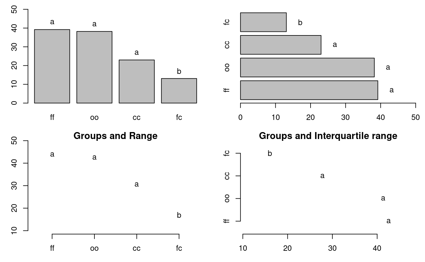
Grouping of treatments and its variation, Median method
par(oldpar)
Durbin
durbin.test; example: Myles Hollander (p. 311) Source: W. Moore and C.I. Bliss. (1942) A multiple comparison of the Durbin test for the balanced incomplete blocks for sensorial or categorical evaluation. It forms groups according to the demanded ones for level of significance (alpha); by default, 0.05.
str(durbin.test)
function (judge, trt, evaluation, alpha = 0.05, group = TRUE, main = NULL,
    console = FALSE)
Analysis
days <-gl(7,3)
chemical<-c("A","B","D","A","C","E","C","D","G","A","F","G", "B","C","F",
"B","E","G","D","E","F")
toxic<-c(0.465,0.343,0.396,0.602,0.873,0.634,0.875,0.325,0.330, 0.423,0.987,0.426,
0.652,1.142,0.989,0.536,0.409,0.309, 0.609,0.417,0.931)
head(data.frame(days,chemical,toxic))
  days chemical toxic
1    1        A 0.465
2    1        B 0.343
3    1        D 0.396
4    2        A 0.602
5    2        C 0.873
6 2 E 0.634out<-durbin.test(days,chemical,toxic,group=FALSE,console=TRUE, main="Logarithm of the toxic dose")
Study: Logarithm of the toxic dose
chemical,  Sum of ranks

  sum
A   5
B   5
C   9
D   5
E   5
F   8
G   5

Durbin Test
===========
Value      : 7.714286
DF 1       : 6
P-value    : 0.2597916
Alpha      : 0.05
DF 2       : 8
t-Student  : 2.306004

Least Significant Difference
between the sum of ranks:  5.00689

Parameters BIB
Lambda     : 1
Treatmeans : 7
Block size : 3
Blocks     : 7
Replication: 3

Comparison between treatments
Sum of the ranks

      difference pvalue signif.
A - B          0 1.0000
A - C         -4 0.1026
A - D          0 1.0000
A - E          0 1.0000
A - F         -3 0.2044
A - G          0 1.0000
B - C         -4 0.1026
B - D          0 1.0000
B - E          0 1.0000
B - F         -3 0.2044
B - G          0 1.0000
C - D          4 0.1026
C - E          4 0.1026
C - F          1 0.6574
C - G          4 0.1026
D - E          0 1.0000
D - F         -3 0.2044
D - G          0 1.0000
E - F         -3 0.2044
E - G          0 1.0000
F - G 3 0.2044 names(out)
[1] "statistics" "parameters" "means"      "rank"       "comparison"
[6] "groups" out$statistics
  chisq.value   p.value  t.value     LSD
     7.714286 0.2597916 2.306004 5.00689